Conversion of wavelengths into RGB values

When we measure light with a spectrometer, we usually obtain intensity-based spectral data over a wavelength range that may also include parts of the visible spectral range (approx. 380–800 nm). Although this data provides precise information about the composition of the light, it does not contain any directly perceptible colors—in other words, we cannot yet see what the light looks like to the human eye from the raw measurements.

raw

Bruton

However, for many applications, especially in the context of visualizations, GUI displays, or interactive learning software, it is very useful to convert spectra in the visible range into color values in the RGB color space. In this way, a computer screen can display the measured colors approximately as they are perceived by humans.

The conversion of spectral data into RGB color values allows, for example

Spectra to be visualized clearly – individual peaks or color mixtures become immediately recognizable;
Interactive user interfaces to be designed in which users can directly compare the color of light sources or materials;
Experiments and measurement results to be presented in a more understandable and intuitive way, e. g., for courses or presentations.

In short, RGB conversion bridges the gap between precise spectral measurement and human color perception. It transforms dry numbers into a vivid image that can be interpreted directly and supports learning or analysis.

Conversion of spectral data to RGB—scientific or practical

The CIE (Commission Internationale de l'Éclairage) standards exist for the scientifically precise conversion of spectral data to color values. The measured spectra are combined with the CIE standard observer functions and standard light sources to calculate the color space coordinates X, Y, Z. These can then be converted into standardized RGB or Lab values. This method provides accurate, reproducible color values, but is often too complex for quick visualizations or simple application examples.

There is a very useful Python library in the field of CIE colorimetry (i. e., the standards of the Commission Internationale de l'Éclairage) called color-science (often simply imported as color). This library implements CIE standards: CIE 1931 XYZ, CIE 1976 u'v', color differences ΔE, metamerism, color temperature calculations, spectral-to-color value transformations, etc. This allows spectral data, such as that from a DIY spectrometer, to be converted into color coordinates, e. g., into xy chromaticity coordinates or into standardized color spaces such as sRGB.

If you would like to learn more about the scientific details, you can attend one of our regular seminars, where you will have the opportunity to learn about the complete CIE conversions in a practical setting and then conduct your own experiments with precise color calculations.

Approximation according to Dan Bruton

For our purposes in the context of DIY spectrometers, however, a clear approximation according to Dan Bruton, which converts wavelengths directly into RGB colors, is sufficient in practice. This method is easy to understand, can be implemented immediately, and makes the colors directly visible on a screen—ideal for demonstrations, GUI displays, or use in the classroom.

The idea here is that R/G/B components are linearly interpolated for individual wavelength ranges, intensity shielding (a targeted attenuation of spectral intensity to produce more realistic screen colors) is applied at the edge of the visible spectrum, and finally a gamma correction is performed. Very easy to implement—delivers plausible screen colors.

Advantage: fast, no tables/integrals. Disadvantage: not CIE-accurate, possibly inaccurate for color comparison/metamerism.

Dan Bruton used the following wavelength ranges:

380–440 nm ➙ Transition from violet to blue
- Below 380 nm, light becomes invisible to humans (UV) ➙ R,G and B = 0
- From 380 to 440 nm, the »R component« increases linearly from 0 to 1, while B = 1 and G = 0 are set
440–490 nm ➙ Transition from blue to cyan
- Blue light becomes increasingly green ➙ G increases linearly from 0 to 1, while R = 0 and B = 1
490–510 nm ➙ Transition from cyan to green
- Blue component decreases linearly from 1 to 0, Green remains 1 and R remains 0
510–580 nm ➙ Transition from green to yellow
- Green remains constant at 1, blue remains constant at 0, but the red component increases linearly from 0 to 1
580–645 nm ➙ Transition from yellow to red
- Rot = 1, Blau = 0, green decreases from 1 to 0
645–780 nm ➙ Red
- Green/blue component = 0, only red remains at 1
- Above 780 nm ➙ IR ➙ invisible.

The limits 380, 440, 490, 510, 580, 645, and 780 nm do not originate from a physical law, but rather from a practical approximation of the visible spectrum perceived by the human eye:

In short, these »boundaries« are empirical breaks in the visible spectrum, allowing for simple linear interpolation between the basic colors. They are therefore not exactly the peak absorptions of the cones in the eye or CIE functions, but rather a practical approximation based on subjective color perception.

Interesting facts about the Bruton variant: The method presented here for converting wavelengths into RGB values was developed by Dan Bruton, a physicist at Texas A&M University. The method was originally based on a Fortran program and was created to generate a spectral display that simulates the color perception of the human eye.

Although the original source is currently unavailable online, the Bruton method continues to be used in various scientific papers and projects. For example, it was used in the study “Performing Calibration of Transmittance by Single RGB-LEDs” by D. Carreres-Prieto et al. to approximate the RGB values for visible wavelengths: Performing Calibration of Transmittance by Single RGB-LED within the Visible Spectrum.

There are also numerous resources based on the Bruton method for implementation in modern programming languages such as Python or R. One example is the R function wavelength2col from the cooltools package, which uses Dan Bruton's original Fortran implementation: search.r-project.org.

Python code for the Bruton approximation

We also use the Bruton approximation in the scripts for our DIY spectrometers because it is easy to implement.

Here is the corresponding function (also available for download):

def wavelength_to_hex_bruton(wavelength, intensity, gamma=0.8):

    #  Approximates the screen color of a wavelength (380–780 nm) with brightness based on the sensor signal.
    #  Parameters:
    #    wavelength : float : Wavelength in nm
    #    intensity  : float : Sensor signal (0–65536)
    #    gamma      : float : Gamma correction (standard 0.8)
    #   
    #    Returns:
    #    str : RGB-Hex string as e.g. '#rrggbb'
    
    # --- Bruton Color assignment ---
    if wavelength < 380 or wavelength > 780:
        R = G = B = 0.0
    elif 380 <= wavelength < 440:
        R = -(wavelength - 440) / (440 - 380)
        G = 0.0
        B = 1.0
    elif 440 <= wavelength < 490:
        R = 0.0
        G = (wavelength - 440) / (490 - 440)
        B = 1.0
    elif 490 <= wavelength < 510:
        R = 0.0
        G = 1.0
        B = -(wavelength - 510) / (510 - 490)
    elif 510 <= wavelength < 580:
        R = (wavelength - 510) / (580 - 510)
        G = 1.0
        B = 0.0
    elif 580 <= wavelength < 645:
        R = 1.0
        G = -(wavelength - 645) / (645 - 580)
        B = 0.0
    else:  # 645–780
        R = 1.0
        G = 0.0
        B = 0.0


    # --- Intensity correction at the spectrum edges ---
    if 380 <= wavelength < 420:
        factor = 0.3 + 0.7*(wavelength - 380)/(420 - 380)
    elif 420 <= wavelength < 701:
        factor = 1.0
    elif 701 <= wavelength <= 780:
        factor = 0.3 + 0.7*(780 - wavelength)/(780 - 700)
    else:
        factor = 0.0


    # --- Logarithmic brightness scale ---
    # Minimum value 1, to avoid log(0) 
    intensity = max(intensity, 1)
    brightness = math.log(intensity) / math.log(65536)  # 0..1
    brightness *= factor  # Factor from Bruton correction


    # --- Gamma correction und 0–255 scaling ---
    def adjust(c):
        return int(round((c * brightness) ** gamma * 255))

    r, g, b = adjust(R), adjust(G), adjust(B)
    return f'#{r:02x}{g:02x}{b:02x}'

As an example, we show here the spectrum of a white light LED lamp, which is visualized using the Bruton approximation. This figure clearly shows that the transitions between the individual colors are represented without any major jumps.

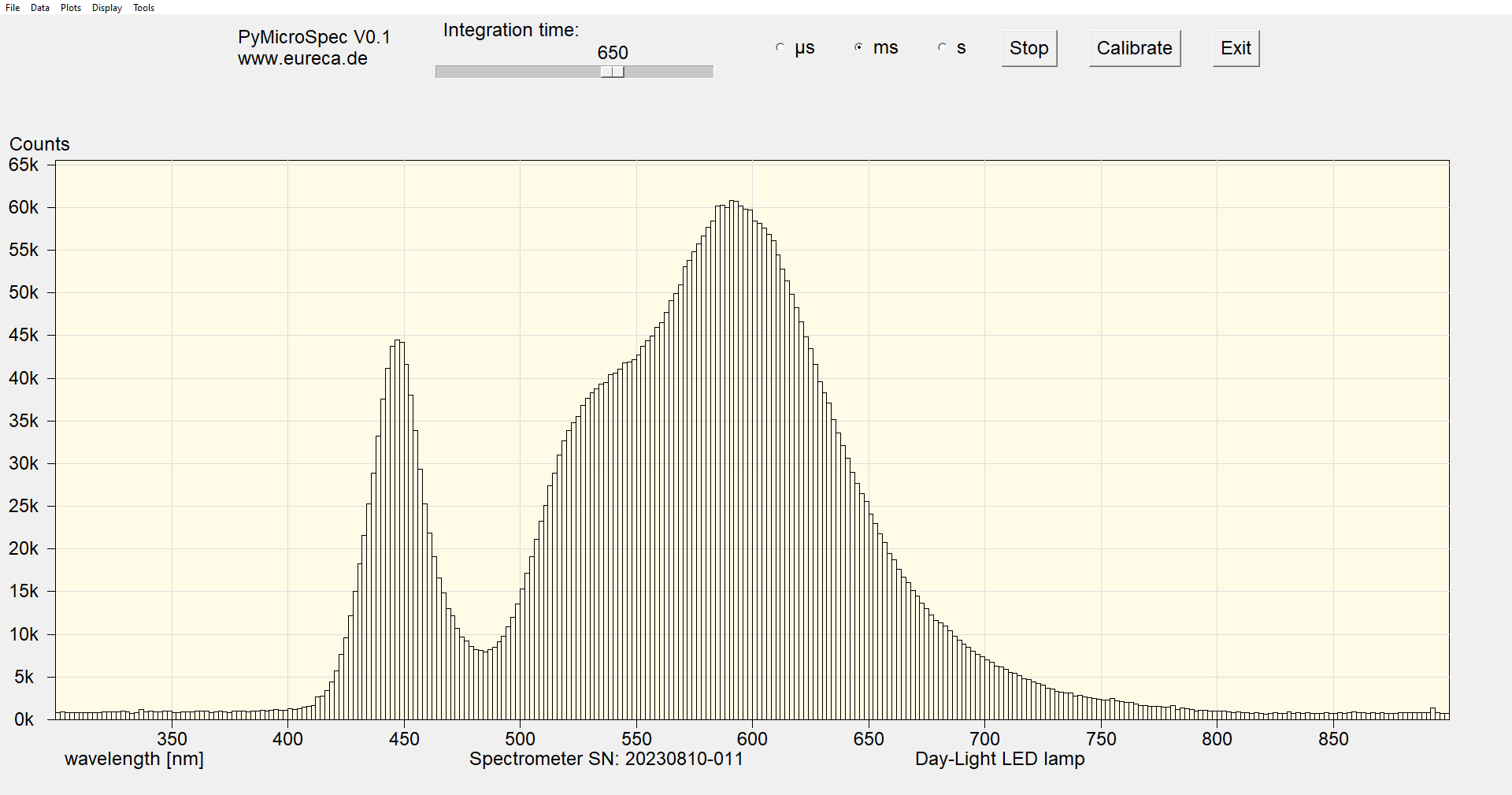
Example illustration of raw spectrum data.

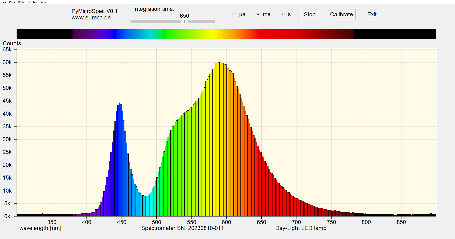
Example illustration of a spectrum with coloring using the Bruton approximation.

Here you can easily ask a question or inquiry about our products:

Product inquiry

Last update: 2025-08-09

Conversion of wavelengths into RGB values

Conversion of spectral data to RGB—scientific or practical

Approximation according to Dan Bruton

Python code for the Bruton approximation

Product inquiry

Request for: