EasyCalibrate Pro

Wavelength calibration of spectrometers using second-order polynomials

In the EasyCalibrate script, we showed how to perform wavelength calibration (i. e., the assignment of pixels ➙ wavelength (nm) for our DIY spectrometers) with just a few lines of Python script. For this purpose, linear regression was used, which is perfectly adequate for simple applications with low calibration requirements.

However, if you want to perform more sophisticated experiments, you will quickly find that linear calibration is not sufficient for this purpose. The use of second-degree polynomials provides a remedy here.

On this page, we present a corresponding improved Python script. With this script, our DIY spectrometers can be calibrated so that, for example, the positions of the emission peaks across the entire sensor area can be determined in the experiment with an accuracy of a few tenths of a nanometer.

Wavelength calibration with red CCFL (cold cathode fluorescent lamp) as reference source

For the demonstration of the script, a red cold cathode lamp (CCFL) is used here as an example reference source, since these light sources are relatively easy and inexpensive to obtain (we are happy to help with this).

They are used, for example, in the effect lighting of gaming PCs or as LCD backlights.

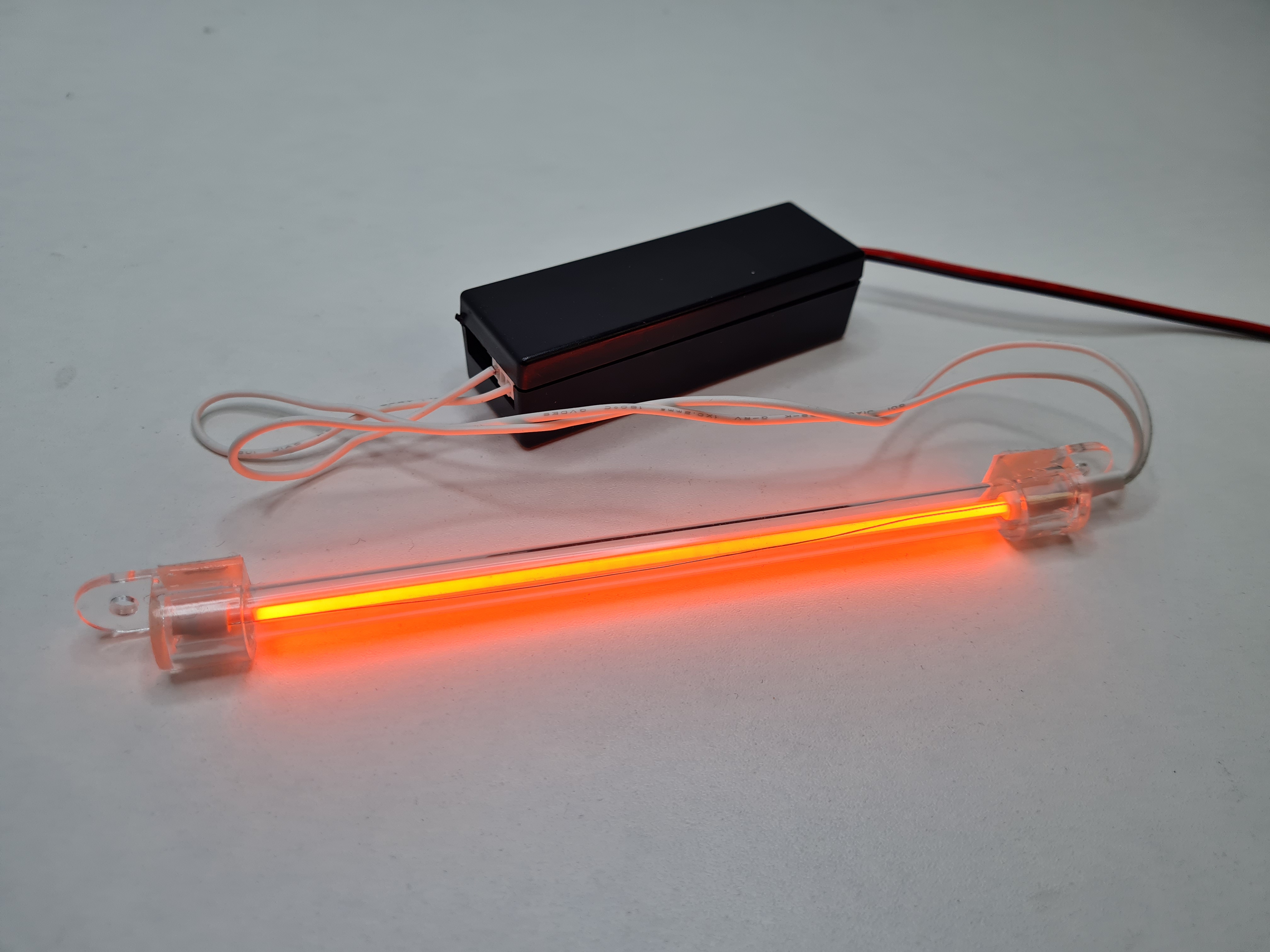
But in general, CCFLs offer a number of additional advantages:

they can be operated with the aid of a battery-powered inverter;
In the start-up phase, CCFLs show several narrow emission lines between 435 nm and 810 nm, which are distributed relatively evenly across the sensitivity range of our DIY spectrometer; this is very practical for reliable and robust polynomial calibration using quadratic fit;
the position of the emission lines is very temperature-stable.

However, other light sources (such as LEDs or laser diodes) with known emission maxima can also be used for calibration. Bandpass or edge filters are also suitable. Some of these options are already prepared (but commented out) in the example script. These can be reactivated at any time if required and modified with the wavelengths and designations specifically used by the user.

Short and compact: What EasyCalibratePro can do

The software provides a live display of the line-scan camera data (counts versus pixel, and after calibration also with a wavelength scale) and allows you to set the integration time as well as start and stop the camera.

Reference peaks can be marked interactively, either via right-click or by pressing the spacebar.

Depending on the number of reference points, a fit is performed for calibration: With two reference points, a linear fit is performed; with three or more reference points, a quadratic fit (2nd order) is performed. The calibration can be saved and reloaded, whereby both a CSV file and a TXT file are generated for compatibility reasons with other scripts. In addition, the currently recorded spectrum can be exported as CSV (pixels, counts, and optionally wavelength).

The workflow explained quickly

Start script
python EasyCalibratePro.py
Switch on CCFL and measure immediately
The argon lines are still present in the first ~20 s.
Stop live readout (Start/Stop)
Live readout is stopped for reproducible peak setting.
Prepare calibration dialog
Open »Start Calibration,« reference buttons are visible.
Select reference ➙ Set peak
Set by right-clicking or pressing the space bar (both are bound).
Calculate fit (Calibrate)
- 2 points: linear
- ≥3 points: quadratic (2nd order)
Save calibration (Save)
A CSV file (a,b,c) and, optionally, a TXT file for older tools are created.

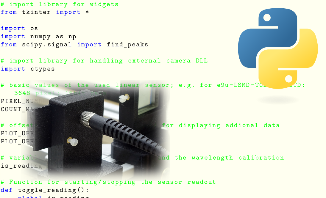
The complete Python script is available for download here. Only the most important passages are discussed in detail below.

Screen video: »Calibration with red CCFL (during the start phase)«

This video shows the workflow when using the script. First, after switching on the lamp, an integration time is selected at which the reference peaks are clearly visible. After stopping the camera, the lines can then be identified and marked at leisure.

Special feature of CCFL calibration: Measurement window approx. 20 seconds.

In the red CCFL, in addition to the Hg lines, Argon lines are also clearly visible at the beginning. These Argon lines are particularly valuable for calibration because they provide additional reference points in the red/NIR range. However, they disappear within about 20 seconds once the lamp reaches operating temperature.

Why? During warm-up, the mercury vapor pressure/concentration in the tube rises; the spectrum becomes increasingly dominated by Hg processes, and Argon emissions fade into the background (depending on the lamp type, this happens faster or slower).

After warm-up, the spectrum is stable, but less attractive for a »multi-point« calibration: The red color now mainly comes from a phosphor that has strong emission around approx. 615 nm and weaker components between approx. 575 – 625 nm; the additional Argon lines are no longer available.

For calibration, the reference lines should therefore be made visible within the first ~20 seconds after switching on by choosing an appropriate integration time, and then the camera should be stopped. In practice, this also means that the calibration script should already be running before the CCFL is turned on.

Calibration quality: Best practices

The quality of a calibration depends primarily on the selected reference peaks and the integration time used!

Be aware of the time window:: The references should be quick and easy to find. Here, for example, set them within the first ~20 s before the argon lines disappear. Use prepared »fingerprints« (see below) of the required signals!
Distribute reference points cleverly:: Do not just calibrate »in the middle«; deliberately include lines at the ends of the measuring range (here, for example: Ar 696/763/810).
Avoid saturation:: Peaks must not be »cut off« at the top because the sensor may be overdriven/saturated; otherwise, the maximum will shift.
Mark peak maximum::: For emission lines, always select the maximum, not an edge. Edges are more suitable when using edge filters.

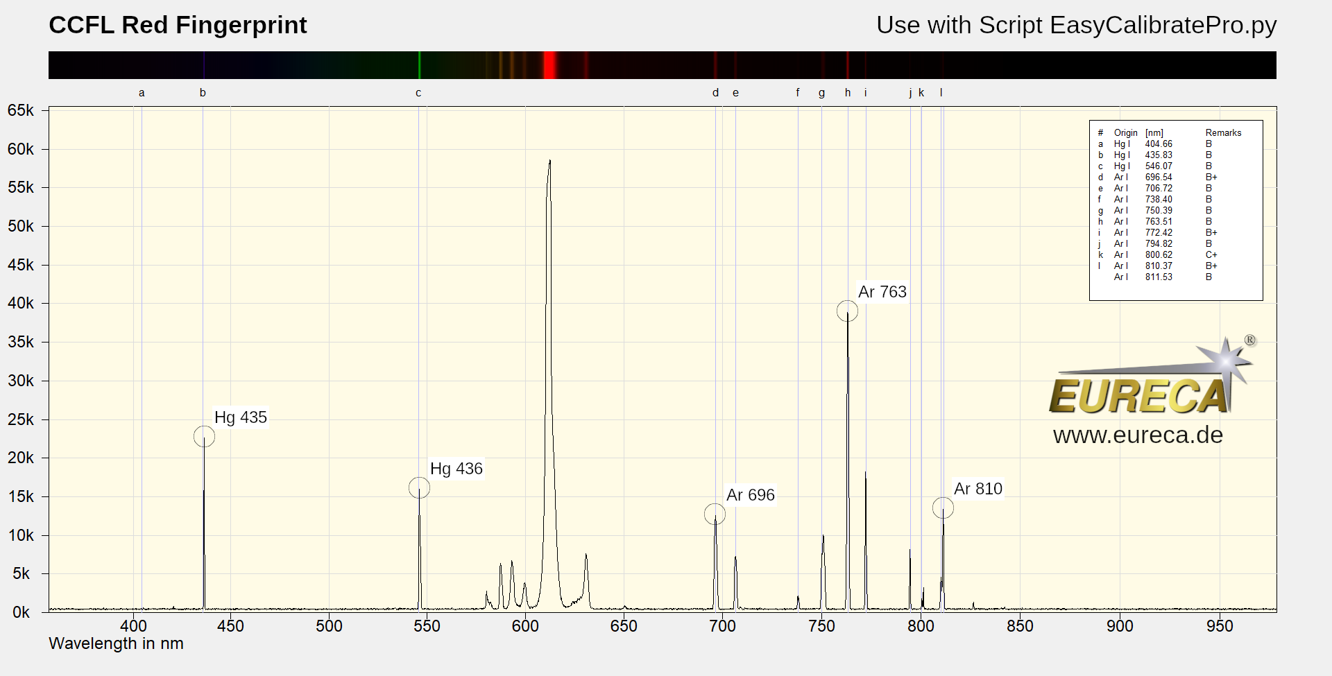
»Spectral fingerprint«: The positions of the emission lines used in the script are marked in this spectrum. Simply click and print: This should make it easy to identify the corresponding lines during calibration.

Reference lines in the script: CCFL (Hg/Ar) as an example configuration

At the beginning of the script, the reference source is selected via a commented-out block. Five reference points are prepared for the red CCFL (Hg/Ar):

# calibration data for five emission lines (Hg/Ar) of a red CCFL (Cold Cathode Fluorescent Lamp)

# number of calibration points (min. 2, max. 5)
N_REF_POINTS = 5  

# wavelengths of the calibartion lines/points
ref_values_nm = [435.83, 546.07, 696.54, 763.51, 810.37][:N_REF_POINTS]

# label of buttons
ref_labels = ["Peak for \"Hg 435\"", "Peak for \"Hg 546\"", "Peak for \"Ar 696\"", "Peak for \"Ar 763\"", "Peak for \"Ar 810\""][:N_REF_POINTS]

The script also already contains (commented out) sections for the use of other reference sources, including for bandpass filters or inexpensive laser diode modules.

Second-order polynomial regression in spectrometer calibration

Why is »linear« often not enough?

Over larger spectral ranges, the »pixel ➙ wavelength« mapping in real setups is often slightly nonlinear (optical geometry, imaging errors, dispersion effects). A quadratic approach is an established, stable compromise here: significantly more accurate than linear, but much more robust than higher polynomials.

Model and fit in the script

A quadratic model is used for three or more reference points:

λ (p x) = a \cdot p x^{2} + b \cdot p x + c

In the code (key lines):

               a, b, c = np.polyfit(pixels, waves, 2)
               polyfit = np.poly1d([a, b, c])

With exactly two points, a linear fit is automatically applied.

From measurement points to calibration curve: What does polynomial regression do?

For wavelength calibration, you need a list of measurement pairs:

Pixel position p (e. g., where is an emission peak on the sensor?)
Wavelength λ in nm (what is the »real« wavelength of this peak?)

For example, $λ (p) = a \cdot p^{2} + b \cdot p + c$ .

We are then looking for a function that converts each pixel $p$ into the best possible wavelength $λ$ :

The following model is often used for a quadratic approach (2nd order polynomial):

λ (p) = a \cdot p^{2} + b \cdot p + c

The three coefficients $a$ , $b$ and $c$ are then exactly what is ultimately stored as calibration data for the spectrometer.

»Best possible« – what does that mean mathematically?

With exactly three reference points, $a$ , $b$ and $c$ can be determined so that the parabola passes exactly through all three points.

In practice, however, there are often more than three reference lines – and then there is generally no parabola that passes perfectly through all points (e. g., due to peak uncertainty, noise, saturation, slightly asymmetrical lines, etc.).

Therefore, the curve that best fits the points on average is typically sought. The standard approach here is the least squares method: the sum of the quadratic deviations (residuals) is minimized.

This is exactly what the np.polyfit(...) function does in the background: a least squares fit for a polynomial of a given degree.

How can you roughly calculate the coefficients »by hand«?

Case A: 3 reference points (exactly determinable)
Set up a linear equation system for $a$ , $b$ and $c$ and solve it (classically, e. g., using Gaussian elimination).
Case B: more than 3 reference points (overdetermined)
Formulate a least squares problem and solve it using least squares. The classic approach uses normal equations or numerically more stable methods (e. g., QR decomposition/SVD, depending on the implementation).

The »cool« thing: Doing this by hand is tedious and prone to numerical errors – Python solves it robustly in milliseconds (and even warns you if the fit is poorly conditioned).

What do $a$ , $b$ and $c$ mean in the context of a spectrometer?

The function

λ (p) = a \cdot p^{2} + b \cdot p + c

is the calibration curve »pixel ➙ nm«.

$c$ (offset): defines the »zero point« of the curve (formally $λ (0)$ ). This is mathematically important, even though pixel 0 is often not in the area of interest.
$b$ (linear dispersion/slope): roughly corresponds to »nm per pixel« if the image is approximately linear.
$a$ (curvature/nonlinearity): describes how much the dispersion varies across the sensor (i. e., how much the mapping deviates from a straight line).

This becomes practically tangible via the local dispersion (derivative):

\frac{d λ}{d p} = 2 a \cdot p + b

This means that for pixel $2 a \cdot p + b$ , the »nm per pixel scaling« is approximately $a$ . This is helpful, for example, when a line width is measured in pixels and interpreted in nm.

Mini rules of thumb for good fits

For second order, at least 3 points are necessary – more is good, as long as the lines are reliable.
Distribute reference lines across the entire sensor area if possible (not just »in the middle«).
Avoid extrapolatingif possible: calibration is most reliable between the reference points.

Note for further reading: A detailed derivation (normal equations, QR/SVD, etc.) can be found very well explained on the internet, e. g. here:

Methode der kleinsten Quadrate [German] or as the English equivalent Least squares
numpy.polyfit
Least squares and the normal equations (PDF)

Here you can easily ask a question or inquiry about our products:

Product inquiry

Last update: 2026-24-02