EasyCalibrate: Spectral calibration of a Spectrometer using a neon lamp

This application note describes the process of the spectral calibration of a spectrometer using the Czerny-Turner Spectrometer CTS-150 as an example. However, this procedure can also be used for other spectrometer types with a similar design. It uses a short Python script called EasyCalibrate, which is an extension of our script EasyDisplay. The script displays the sensor data graphically and uses the manual identification of characteristic peaks in the spectrum of a neon lamp for the calibration process.

A spectrometer uses an optical diffraction element (e. g. a grid or prism) to separate the different wavelengths in a light signal. A line scan camera is often used to detect the separated wavelengths. Depending on the optical arrangement, each pixel position corresponds to a specific wavelength range.

To calibrate a spectrometer, you need to know the correlation between the pixel position and the wavelength of the signal. A simple calibration method, which is nevertheless suitable for most basic applications, is to use a signal from a known light source with narrow emission lines. Such lines with known and fixed wavelengths are emitted by neon lamps, for example.

Requirements

Sie benötigen ein Czerny-Turner-Spektrometer CTS-150, eine Glimmlampe mit bekannten Peaks sowie einen Computer mit dem Skript EasyCalibrate. Einzelheiten zum Herunterladen und Installieren des Python-Skripts auf Ihrem Computer finden Sie in der Dokumentation für das Skript EasyDisplay.

Glimmlampen sind sehr billige Bauteile, die z. B. noch als Statuslampen in elektronischen Geräten oder Schaltsteckern verwendet werden. Das Spektrum dieser Bauteile zeigt ein charakteristisches Peakmuster im Wellenlängenbereich zwischen 580 nm und 710  m. In diesem Bereich sind etwa 22 Peaks mit unterschiedlichen Stärken sichtbar.

Wir bieten geeignete Kalibriermodule an, die auch als Bausatz selbst aufgebaut werden können. Details zur Gewinnung des Spektrums einer Glimmlampe finden Sie in unserem Applikationsbeispiel Spektroskopie an Glimmlampen.

You will need a Czerny-Turner spectrometer CTS-150, a neon lamp with known peaks and a computer with the script EasyCalibrate. For details on how to download and install the Python script on your computer, see our documentation for the EasyDisplay script.

Neon lamps are very cheap components that are still used, for example, as status lamps in electronic devices or switch plugs. The spectrum of these components shows a characteristic peak pattern in the wavelength range between 580 nm and 710 nm. Around 22 peaks with different strengths are visible in this range.

We provide suitable calibration modules, which can also be assembled as a kit. Details on obtaining the spectrum of a neon lamp can be found in our application example Spectroscopy on Neon Lamps.

Calibration process

Make sure that the line scan camera of the Czerny-Turner spectrometer is correctly connected to the computer and start the script EasyCalibrate. Switch on the neon lamp, let it warm up for one minute and bring the spectrometer’s light guide input as close as possible to the lamp. If you are using an illumination or calibration module, you can simply connect the light guide to the corresponding light source output. You should now see the characteristic peaks of the neon spectrum on your computer screen.

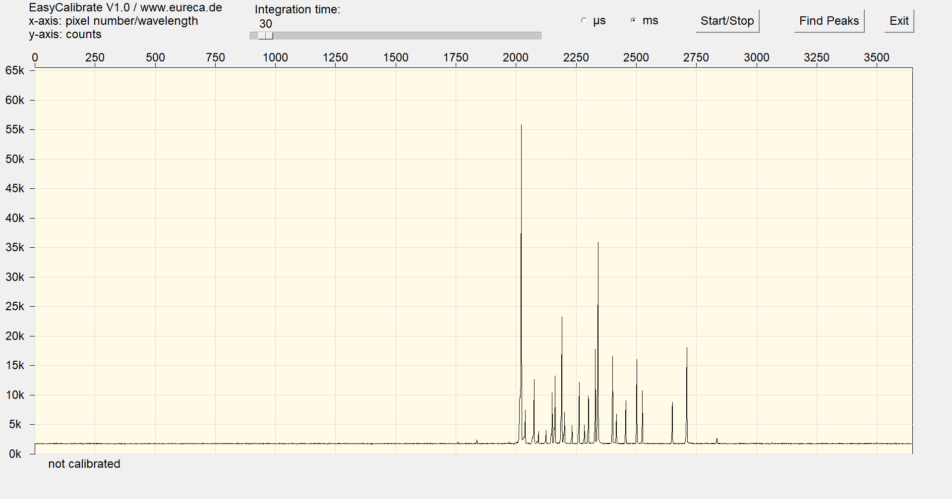
Spectrum of a neon lamp, recorded with uncalibrated spectrometer

The script uses an external text file named EasyCalibrate.config to store calibration data already obtained. If you run the script for the first time and this file does not exist, the x-axis of the signal plot will be labeled »not calibrated«. If the calibration data file is found, the x-axis will be labeled with the corresponding wavelengths calculated from the saved calibration values.

Now set the integration time so that the largest peak of the spectrum has a height of approx. 55k counts. With such an integration time, the sensor signal is not distorted by possible saturation effects, which can occur at higher intensities, and the peaks can be found more reliable by the script.

Press the »Find Peaks« button and a new window will open, listing the peaks found. If the spectrometer has not yet been calibrated, only the peak number, the pixel position and the maximum number of peaks are displayed in this list. The respective wavelength is then displayed with a dash: »-«.

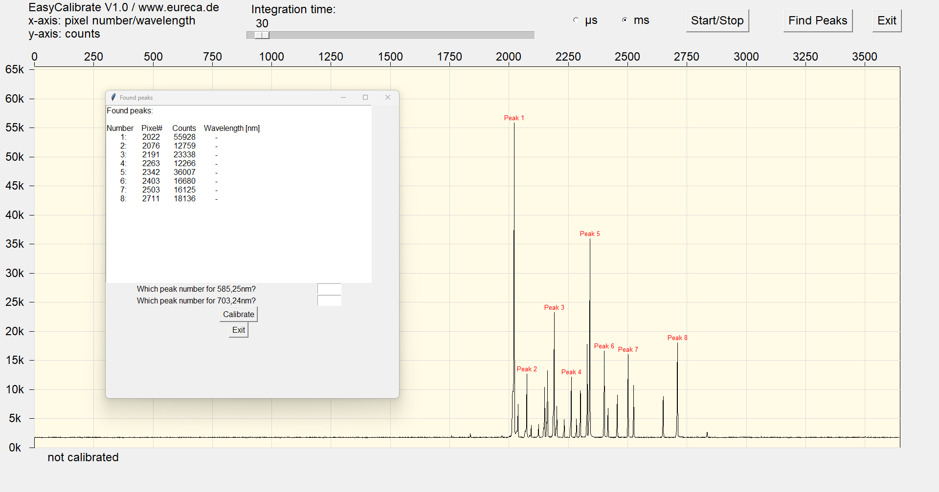
Spectrum with found an numbered peaks

The Peak detection is performed by the script using the find_peaks function of the SciPy module, which is very powerful and easy to use at the same time. In addition to listing the peaks, the corresponding signals in the spectrum are also assigned numbers for reference purposes.

For the calibration, the script uses the neon peaks at 585.25 nm and 703.24 nm, which we will call calibration peaks here. These calibration peaks are quite easy to find as they are both the first and the last high signal of the peak series. Depending on the production batch of the lamp and the supply voltage used, the height of the individual peaks may vary slightly, but the calibration peaks are normally so dominant that they can hardly be confused. However, the tolerances in the peak heights can influence the order in which the individual peaks are found and labeled by the script.

If you use a different light source to calibrate the spectrometer, you may need to change the wavelengths used for the calibration peaks in the script.

There are two input fields below this list with the peaks found. The peak number for the calibration peaks can be entered here. In the example shown, these are the numbers #1 and #8. After pressing the »Calibrate« button, the script performs a linear regression based on the positions of the reference peaks and calculates the resolution of the spectrometer and the offset, i. e. the wavelength for the first sensor pixel. These two values will now be used to calibrate the x-axis and the corresponding markers are drawn in.

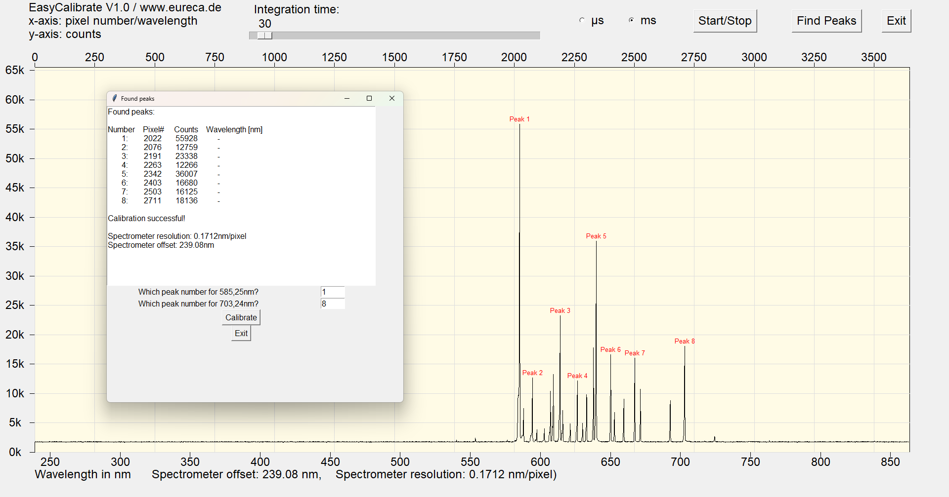
Calibrated spectrum

After calibrating the spectrum, you can press the »Find Peaks« button again at any time to find new peaks in the current sensor signal. The calculated wavelengths are now also listed for the peaks found. This function can therefore also be used to measure unknown peaks.

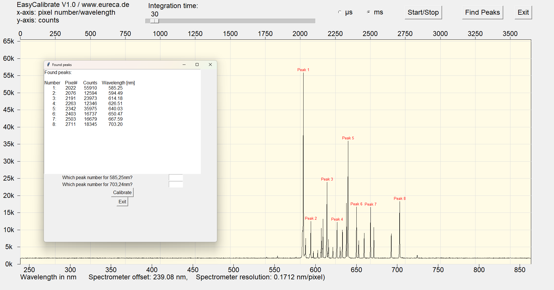
List of found peaks with calculated wavelengths

EasyCalibrate Python Code

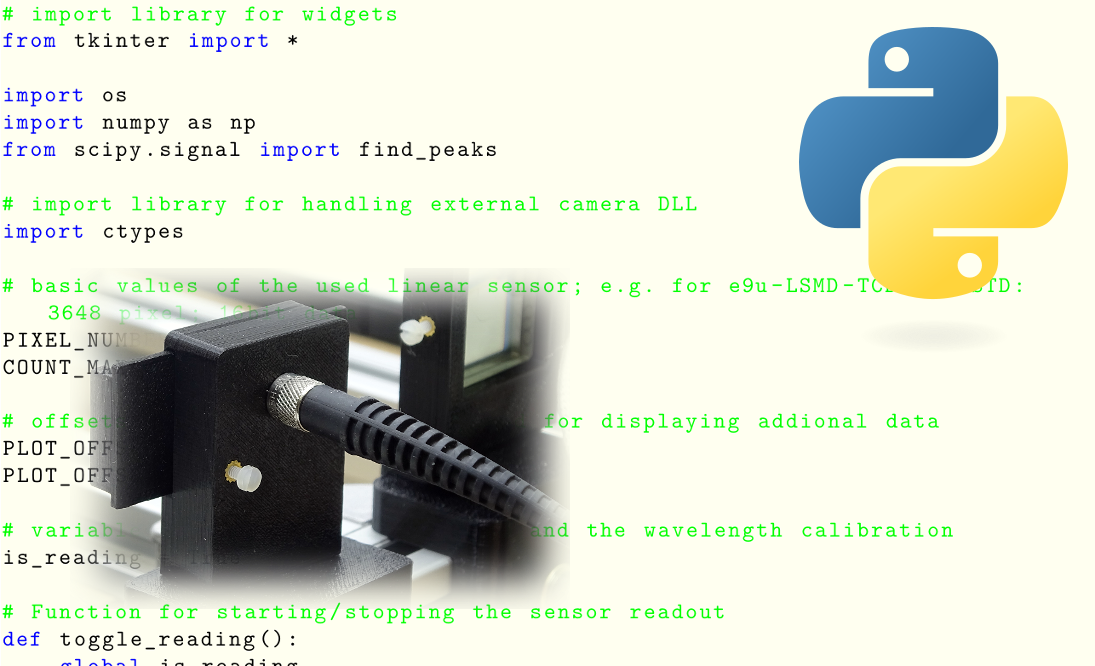
# EasyCalibrate.py V1.1
#
# Python display tool for line scan cameras by EURECA Messtechnik GmbH 
# - detects the camera via the EasyAccess DLL
# - reads out the camera and displays the recorded sensor data
# - integration time can be adjusted between 1µs and 1000ms
#
# For details please refer to: www.eureca.de

# import library for widgets
from tkinter import *

import os
import numpy as np
from scipy.signal import find_peaks

# import library for handling external camera DLL
import ctypes

# basic values of the used linear sensor; e.g. for e9u-LSMD-TCD1304-STD: 3648 pixel; 16bit data
PIXEL_NUMBER = int(3648)
COUNT_MAX = int(65536)

# offsets for the plot window; needed for displaying addional data
PLOT_OFFSETX = 70
PLOT_OFFSETY = 50

# variable to test the camera status and the wavelength calibration
is_reading = True

# Function for starting/stopping the sensor readout
def toggle_reading():
    global is_reading
    is_reading = not is_reading

def Plot_Sensordata_Wavelength():

# axis marking for wavelength
  wavelength_start = spectrometer_offset
  wavelength_end = spectrometer_offset + 3648*spectrometer_resolution

  plot.delete("wavelength")

  for x in range(100,1200,50):
    if (x > wavelength_start) and (x < wavelength_end):

# print(x)

# print(wavelength_to_pixel(x))
      
      plot.create_line(PLOT_OFFSETX + wavelength_to_pixel(x)*plot_width/PIXEL_NUMBER, plot_height + PLOT_OFFSETY, PLOT_OFFSETX + \
                       wavelength_to_pixel(x)*plot_width/PIXEL_NUMBER, plot_height + PLOT_OFFSETY + 10, tags="wavelength") 
      plot.create_text(PLOT_OFFSETX + wavelength_to_pixel(x)*plot_width/PIXEL_NUMBER, plot_height + PLOT_OFFSETY + 20, font=("Arial Bold", 18),text=str(x),fill='black', \
                       tags="wavelength")

  spectrometer_offset_output = "Spectrometer offset: " + str(spectrometer_offset) + str(" nm")
  spectrometer_resolution_output = "Spectrometer resolution: " + str(spectrometer_resolution) + str(" nm/pixel")
  wavelength_output ="Wavelength in nm      " + spectrometer_offset_output + ",    " + spectrometer_resolution_output + ")"
  plot.create_text(PLOT_OFFSETX, plot_height + PLOT_OFFSETY + 45, font=("Arial Bold",18),text=wavelength_output,fill='black', tags="wavelength", anchor="w")

# calibrate the spectrometer using the two choosen peaks from the neon spectrum
def calibrate_sensor():
      
    global spectrometer_offset, spectrometer_resolution

# get the wavelengths of the two choosen peaks 
    wavelength_1 = peaks[int(peak_num_entry.get())-1]
    wavelength_2 = peaks[int(peak_num_entry2.get())-1]

# calculate the spectrometer resolution in nm/pixel
    spectrometer_resolution = round((703.24 - 585.25) /  (wavelength_2 - wavelength_1),4)

# calculate the offset of the spectrometer, which is defined as the wavelength at the first pixel
    spectrometer_offset = round(585.25 - wavelength_1 * spectrometer_resolution,2)

    output_text.insert(END, "\nCalibration successful!\n\n")
    output_text.insert(END, "Spectrometer resolution: " + str(spectrometer_resolution) + "nm/pixel")
    output_text.insert(END, "\nSpectrometer offset: " + str(spectrometer_offset) +"nm")

    is_calibrated = True
    Plot_Sensordata_Wavelength()

# writing configuration file
    file = open("EasyCalibrate_config.txt", "w")
    file.write("spectrometer_offset " + str(spectrometer_offset) + "\n")
    file.write("spectrometer_resolution " + str(spectrometer_resolution))
    file.close() 

def wavelength_to_pixel(wavelength):
  
  global spectrometer_offset, spectrometer_resolution

# print(wavelength)
  pixel = (wavelength - spectrometer_offset) / spectrometer_resolution

# print(pixel)
  return pixel

def close_peak_window():

  plot.delete("peaks")
  peak_window.destroy()

def find_and_show_peaks():

    global peaks, peak_num_entry, peak_num_entry2, output_text, peak_window

# Receive sensor values
    sensor_data = [pointer[pixel] for pixel in range(PIXEL_NUMBER)]

# Finding peaks with the find_peaks function of SciPy
    peaks, _ = find_peaks(sensor_data, height=10000, distance=50)

# Create a new window for the output of the peaks found
    peak_window = Toplevel(master)
    peak_window.title("Found peaks")
    peak_window.geometry("600x600")

# Text field for displaying the peaks found
    output_text = Text(peak_window, font=("Arial", 12), width=60, height=20)
    output_text.grid(row=0, column=0, columnspan=2)

# Entry fields for peak numbers
    peak_num_label = Label(peak_window, text="Which peak number for 585,25nm?", font=("Arial", 12))
    peak_num_label.grid(row=1, column=0)
    peak_num_entry = Entry(peak_window, font=("Arial", 12), width=5)
    peak_num_entry.grid(row=1, column=1)

    peak_num_label2 = Label(peak_window, text="Which peak number for 703,24nm?", font=("Arial", 12))
    peak_num_label2.grid(row=2, column=0)
    peak_num_entry2 = Entry(peak_window, font=("Arial", 12), width=5)
    peak_num_entry2.grid(row=2, column=1)

# Calibration button
    calibrate = Button(peak_window, text="Calibrate", font=("Arial", 12), command=calibrate_sensor)
    calibrate.grid(row=3, column=0, columnspan=2)

# Button for closing the window
    exit_button = Button(peak_window, text="Exit", font=("Arial", 12), command=close_peak_window)
    exit_button.grid(row=4, column=0, columnspan=2)

# Output of the peaks found in the text field
    output_text.insert(END, "Found peaks:\n\nNumber    Pixel#     Counts    Wavelength [nm]\n")
    for idx, peak_index in enumerate(peaks):
        wavelength = spectrometer_offset + peak_index * spectrometer_resolution
        if wavelength > 0:
          output_text.insert(END, f"{idx+1:>8}:       {peak_index:>5}       {sensor_data[peak_index]:>5}          {wavelength:6.2f}\n")
        else:
          output_text.insert(END, f"{idx+1:>8}:       {peak_index:>5}       {sensor_data[peak_index]:>5}          -\n")

# Update plot and number peaks consecutively
    for idx, peak_index in enumerate(peaks):
        counts = sensor_data[peak_index]
        x = int(peak_index / PIXEL_NUMBER * plot_width)
        y = int(counts / COUNT_MAX * plot_height)

        # Update plotting of the peak marker above the PeakPlot and number peaks consecutively
        plot.create_text(x + PLOT_OFFSETX, plot_height + PLOT_OFFSETY - y - 10, 
                         font=("Arial", 10), text=f"Peak {idx+1}", fill="red", tags="peaks")

print("EasyCalibration V1.1\nSearching for camera: ")

# open external DLL
libe9u = ctypes.WinDLL('./libe9u_LSMD_x64.dll')

# define argument and return types for the used functions
libe9u.e9u_LSMD_search_for_camera.argtype = ctypes.c_uint
libe9u.e9u_LSMD_search_for_camera.restype = ctypes.c_int

libe9u.e9u_LSMD_start_camera_async.argtype = ctypes.c_uint
libe9u.e9u_LSMD_start_camera_async.restype = ctypes.c_int

libe9u.e9u_LSMD_set_times_us.argtypes = (ctypes.c_uint, ctypes.c_uint, ctypes.c_uint)
libe9u.e9u_LSMD_set_times_us.restype = ctypes.c_int

libe9u.e9u_LSMD_get_next_frame.argtype = ctypes.c_uint
libe9u.e9u_LSMD_get_next_frame.restype = ctypes.c_int

libe9u.e9u_LSMD_get_pixel_pointer.argtypes = (ctypes.c_uint, ctypes.c_uint)
libe9u.e9u_LSMD_get_pixel_pointer.restype = ctypes.POINTER(ctypes.c_uint16)

# Seach for a suitable camera on all USB ports and quit with returning the error code, if no camera is found
i_status = libe9u.e9u_LSMD_search_for_camera(0)
if i_status != 0:
  print("No camera found! Error Code: " + str(i_status))
  exit(1)

print("Starting camera: ", end='')
libe9u.e9u_LSMD_start_camera_async(0)

# getting the pointer to the array containing the sensor data
pointer = libe9u.e9u_LSMD_get_pixel_pointer(0, 0)

# defining the master window for graphical output
master = Tk()

# getting the size of the master window
screen_width = master.winfo_screenwidth()
screen_height = master.winfo_screenheight()

# setting the size of the display window to cover nearly the complete screen
master.geometry(str(screen_width - 50) + "x" + str(screen_height - 100) + "+10+20")

# defining the dimensions for the plot area
plot_width = screen_width - 150
plot_height = screen_height - 300

# defining and packing the control/output widgets
statusline = Frame(master)
statusline.pack(side='top')
plot = Canvas(master)
plot.pack(side ='bottom', fill=BOTH, expand=YES)

# output label for program name and version number
output_peak_width = Label(statusline, text="EasyCalibrate V1.1 / www.eureca.de\nx-axis: pixel number/wavelength\ny-axis: counts", justify=LEFT, font=("Arial Bold", 18))
output_peak_width.pack(side='left', padx=0)

# defining slider for integration time and setting it to 10
faktor = IntVar()
slider_exp_time = Scale(statusline, from_=1, to=1000, length=plot_width/3, orient=HORIZONTAL, label="Integration time:", font=("Arial Bold", 18))
slider_exp_time.pack(side='left', padx=50)
slider_exp_time.set(100)

# defining two radio buttons for switching the integration time between µs and ms
Radiobutton_us = Radiobutton(statusline, text="µs", font=("Arial Bold", 18), variable=faktor, value=1)
Radiobutton_us.pack(side='left', padx=20)
Radiobutton_us.invoke()
Radiobutton_ms = Radiobutton(statusline, text="ms", font=("Arial Bold", 18), variable=faktor, value=1000)
Radiobutton_ms.pack(side='left', padx=20)

start_stop_button = Button(statusline, text="Start/Stop", font=("Arial Bold", 18), command=toggle_reading)
start_stop_button.pack(side='left', padx=50)

find_peaks_button = Button(statusline, text="Find Peaks", font=("Arial Bold", 18), command=find_and_show_peaks)
find_peaks_button.pack(side='left', padx=20)

# defining the exit button with the closing function
def close_window():
    master.destroy()
exit_button = Button(statusline, text="Exit", font=("Arial Bold", 18), command=close_window)
exit_button.pack(side='left', padx=20)

# drawing a rectangular frame for the sensor data
Sensor_Plot = plot.create_rectangle(PLOT_OFFSETX, PLOT_OFFSETY, plot_width + PLOT_OFFSETX, plot_height + PLOT_OFFSETY, fill="#fffbe6")

# x-axis marking with pixel number
for x in range(15):
  plot.create_line(PLOT_OFFSETX + x*250*plot_width/PIXEL_NUMBER, PLOT_OFFSETY, PLOT_OFFSETX + x*250*plot_width/PIXEL_NUMBER, PLOT_OFFSETY - 10)
  plot.create_text(PLOT_OFFSETX + x*250*plot_width/PIXEL_NUMBER, PLOT_OFFSETY - 20,font=("Arial Bold", 18),text=int(x*250),fill='black')

  plot.create_line(PLOT_OFFSETX + x*250*plot_width/PIXEL_NUMBER, PLOT_OFFSETY, PLOT_OFFSETX + x*250*plot_width/PIXEL_NUMBER, PLOT_OFFSETY + plot_height, fill="#dddddd")

# y-axis marking with count number
for y in range(14):
  plot.create_line(PLOT_OFFSETX-10, PLOT_OFFSETY + plot_height - y*5000*plot_height/COUNT_MAX, 
                   PLOT_OFFSETX, PLOT_OFFSETY + plot_height - y*5000*plot_height/COUNT_MAX)
  text_output = str(y*5) + "k"
  plot.create_text(PLOT_OFFSETX-40, plot_height + PLOT_OFFSETY - y*5000*plot_height/COUNT_MAX,font=("Arial Bold", 18),text=text_output,fill='black')

  plot.create_line(PLOT_OFFSETX + plot_width, PLOT_OFFSETY + plot_height - y*5000*plot_height/COUNT_MAX, 
                   PLOT_OFFSETX, PLOT_OFFSETY + plot_height - y*5000*plot_height/COUNT_MAX, fill="#dddddd")

spectrometer_offset = 0.0
spectrometer_resolution = 0.0

# check if there is a cofiguration file in the same directory
if os.path.exists("EasyCalibrate_config.txt"):

# reading configuration file, values indicated here will overwrite the default values
  file = open("EasyCalibrate_config.txt", "r")
  for line in file:
    config_variable = line.split()[0]
    config_value = line.split()[1]

# print(str(config_variable) + " = " + str(config_value))

# if config_variable == "spectrometer_name":

#  spectrometer_name = config_value
    if config_variable == "spectrometer_offset":
      spectrometer_offset = float(config_value)
    if config_variable == "spectrometer_resolution":
      spectrometer_resolution = float(config_value)

  file.close()

# print the sensor wavelength at the lower side of the plot window
  Plot_Sensordata_Wavelength()
else:
  plot.create_text(PLOT_OFFSETX + 100, plot_height + PLOT_OFFSETY + 20, font=("Arial Bold", 18),text="not calibrated",fill='black', tags="wavelength")

def update_plot():
  if not master.winfo_exists():
    return

  if is_reading:

# getting the integration time from the slider and using this value for the exposure time as well as for the frame time
    exposure_time = int(slider_exp_time.get()) * faktor.get()
    frame_time = exposure_time;

# reading out the camera; for details refer to the EasyAccess documentation
    libe9u.e9u_LSMD_set_times_us (0, exposure_time, frame_time)
    libe9u.e9u_LSMD_get_next_frame (0)

    x_old = 0
    y_old = 0

# deleting the old data points
    plot.delete("data")
 
    for pixel in range(0, PIXEL_NUMBER):

        counts = pointer[pixel]

# scaling the sensor data to fit into the plot region
        x = int(pixel / PIXEL_NUMBER * plot_width)
        y = int(counts / COUNT_MAX * plot_height)

# plotting the data point via connecting the current data with the last one
        plot.create_line(x_old + PLOT_OFFSETX,plot_height + PLOT_OFFSETY - y_old,x + PLOT_OFFSETX,plot_height + PLOT_OFFSETY - y, tags="data")
 
        x_old = x
        y_old = y
  
    plot.update()

  master.after(1, update_plot)

update_plot()

master.mainloop()

You will also find this information handy for printing in this PDF.

Here you can easily ask a question or inquiry about our products:

Product inquiry

Last update: 2024-14-02

EasyCalibrate: Spectral calibration of a Spectrometer using a neon lamp

Requirements

Calibration process

EasyCalibrate Python Code

Product inquiry

Request for: